
Time series assessment in the era of Stockholm Convention & GMP
Interactive publication
|
R source code
|
Interactive examples
|
Authors
|


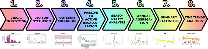
Eight steps of data analysis
Direct links to examples based on R + Shiny
 2: Treatment of values under LoQ |
 3: Outliers exclusion |
 4: Passives recalculation |
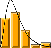
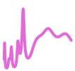
 1: Visual inspection |
|
2: Treatment of values under LoQ |
3: Outliers exclusion |
4: Passives recalculation |
 5: Seasonality analysis |
|
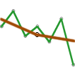
3: Outliers exclusion |
4: Passives recalculation |
5: Seasonality analysis |
 6: Annual aggregation |
|
4: Passives recalculation |
5: Seasonality analysis |
6: Annual aggregation |
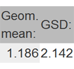 7: Descriptive statistics |
|
5: Seasonality analysis |
6: Annual aggregation |
7: Descriptive statistics |
 8: Trend analysis |
|
1: Visual inspection |
6: Annual aggregation |
7: Descriptive statistics |
8: Trend analysis |
|
2: Treatment of values under LoQ |
1: Visual inspection |
7: Descriptive statistics |
8: Trend analysis |
|
2: Treatment of values under LoQ |
3: Outliers exclusion |
1: Visual inspection |
8: Trend analysis |